Sharpened Cosine Similarity: Part 2
A lot has happened since my last post on the Sharpened Cosine Similarity layer. In this post I will try to give you a quick overview over the most important developments around this feature extractor that shapes up to be more and more interesting.

As described in my previous post in 2020 Brandon Rohrer published a tweet describing how convolutions are a pretty bad feature extractor and offered the idea for an alternative in the shape of a formula and some descriptive gifs:
$$ scs(s, k) = sign(s \cdot k)\Biggl(\frac{s \cdot k}{(\Vert{s}\Vert+q)(\Vert{k}\Vert+q)}\Biggr)^p $$
While this tweet got quite some attention, interestingly nobody seems to have tried the idea out until early 2022 when I stumbled onto the tweet and decided to implement it in the form of a Tensorflow layer. See more on that in my previous post.
The race to them bottom of MNIST:
While implementing the layer I experimented with MNIST and found out that it was super efficient in terms of parameters. Among other interesting properties I discovered that without much effort I was able to reach 99% in MNIST while using only ~3000 parameters. After implementing depthwise Sharpened Cosine Similarity I even managed to do it with less than 1400 parameters which to the best of my knowledge is still a record.
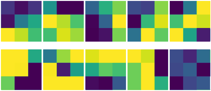
During this race to the bottom of parameter efficiency I had a look at what the network actually learned and could verify that SCS (Sharpened Cosine Similarity) produces very interpretable feature maps. Especially in the first layer it is easy to see edges and significant features in the learned parameters and their activations:

Looking at these activations, it immediately struck me that this layer was not only able to extract exact matches of the features it was looking for but also their opposites. These opposite features would then be represented by negative activations. This also meant that the MaxPooling layer traditionally used to spatially reduce features would only pick up half of the important information.
Once I realized that I decided to implement an AbsMaxPooling Layer that should output the maximum absolute value in the inputs. This turned out to be a huge improvement and further helped to improve results.
The reason for starting the SCS exploration with MNIST was, that the layer is so new and behaves so differently than convolutions that I needed to get a feeling for how it behaves in different situations. For this MNIST was perfect since it allows for lightning fast turnaround times during exploration. This showed me that SCS has some amazing properties:
- SCS can deal with unscaled inputs.
- SCS needs no activation functions.
- SCS needs no normalization layers.
After the initial success with SCS I wanted to move from MNIST to more challenging datasets but unfortunately the first itearations on them did not go as smooth as expected. For a moment that made me doubt the layer as a whole. Despite implementing some complex variants using grouped SCS and soft cosine similarity but the results did not seem to improve. Furthermore I was not able to get the new implementation to run on TPU which made it difficult to do a lot of tests on it.
After struggling with these problems for weeks I finally realized that some of the tweaks I had made in order to reduce the parameter count in my MNSIT experiments had actually hurt the performance on harder datasets. After fixing these tweaks and moving back to the basics to my relief network performed as expected again.
In the meantime also others reported great results using astonishingly simple network architectures.
As an example below you can see a model that with some augmentations and learning rate tricks can reach above 80% on CIFAR-10:
model = tf.keras.Sequential(
    [
        tf.keras.layers.InputLayer(input_shape=input_shape),
        CosSim2D(3, 32),
        MaxAbsPool2D(2, True),
        CosSim2D(3, 64,),
        MaxAbsPool2D(2, True),
        CosSim2D(3, 128),
        MaxAbsPool2D(2, True),
        tf.keras.layers.Flatten(),
        tf.keras.layers.Dense(num_classes)
    ]
)
The Next Steps:
The intriguing properties and its open development has created quite some buzz around the Sharpened Cosine Similarity idea. Apart from my Tensorflow version by now there are also multiple PyTorch implementations.
I'm currently still doing experiemnts on CIFAR but it won't take long until somebody produces the first results on ImageNet.
While the layer mechanics and the basic network components seem to work quite relibly by now, big network architectures have yet to be developed. Personally I'm sure that is only a question of time.
What is clear is that in the case of SCS the open development has had a huge positive impact on the results so I invite you to play with the code yourself and feel free to share your thoughts, ideas or implementations.
If you want to publish something on SCS I invite you to cite the first blog-post until there is a proper paper about it.
@misc{pisoni2022sharpenedcossim,
      title={Sharpened Cosine Distance as an Alternative for Convolutions},
      author={Raphael Pisoni},
      year={2022},
      note={\url{https://rpisoni.dev/posts/cossim-convolution/}},
}