Decoupling Features and Classes with Self-Organizing Class Embeddings
Classification with neural networks is weird! There, I said it!
We usually have a single output per class, as if for some reason each class was it's own feature. The numbers these outputs produce are then intepreted as a log-probability distribution over all the available classes. Eveybody knows it doesn't make sense, yet we treat it as a mathematical assumption. Also needing a separate output for every single class becomes insanely wasteful once you train for more than a few thousand classes. If you have a small model your output layer might well be bigger than the rest of the network.
You can at least get around the huge amount of outputs with some embedding based method by beheading a pretrained network or by doing some contrastive training, but the similarities you get out of them are hard to interpret and you have no measure of certainty.
So what can we do about it you ask? I collected a few ideas...
The Basics
When I think about a class of objects I mostly think about their features and how much they coincide with the class itself.
If something has four legs, is fluffy and has a dangling tounge it's probably a dog.
But not all dogs have four legs, not all of them have fluffy fur and sometimes even the happiest dog has it's mouth shut. Does that make them less of a dog? No.
So it's important to note that while classes might be identifiable by their features, each feature might not apply to that class all the time and at the same time the feature might apply to other classes as well. Thinking about multiple features and classes in that way gets messy pretty soon so let's try to break it down to some easier cases.
\(1\) feature, \(1\) class:
As mentioned above features might not allways apply to a class but they can still be a pretty stong indicator for the class if they are present (middle example). On the other hand features might not be perfect indicators for the class at all and could actually peak for completely different classes that currently lie out of our scope (right example). A third case could be one where a feature is not very indicative for a class, either because it doesn't have a stong peak or because it always applies to a certain degree (left example).
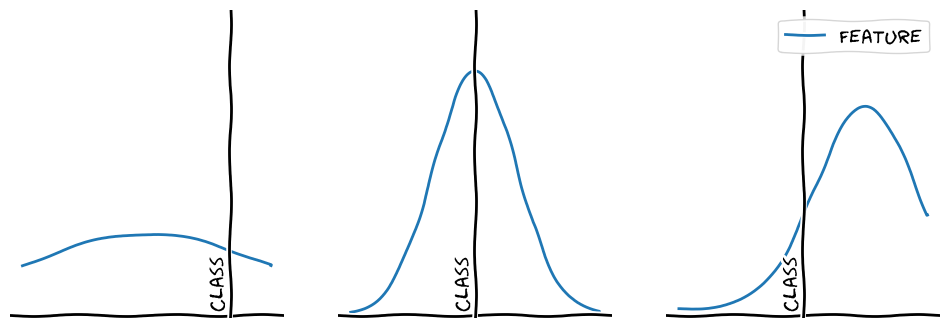
All of those cases show us again that features and classes can be treated as independent things. The same feature can indicate multiple classes and even indicate different classes depending on its strength which we will show in the next example.
\(1\) feature, \(n\) classes:
Nowadays in classification with neural networks we usually learn one feature per class at the model output. So for example we have one feature for "catness" and one feature for "dogness". But as we've seen before, this is not necessary. We don't explicitly need two features to represent two classes if we have some information about the classes themselves. And if we want, we can simply learn this class-information from our training data as well.
We can learn an arbitrary amount of features and classify the samples based on how similar they are to our learned class distributions in the feature space.
As a result below we can see that we can represent two classes with a single feature just fine if we know where on the feature scale the classes are located and how their distribution is shaped.
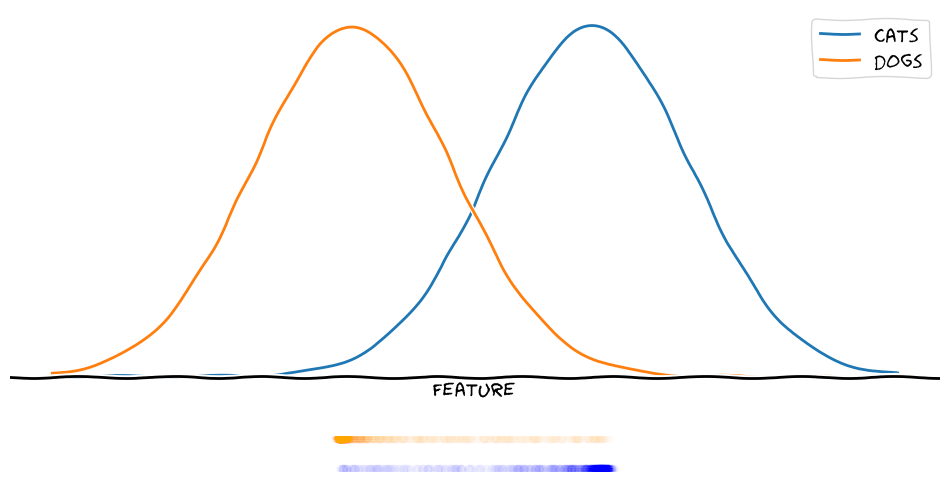
For two classes this is of course possible with other methods as well, but with the method I propose, it generalizes to any combination of \(n\) classes and \(m\) features.
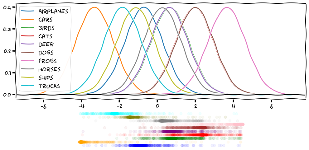
Below you can see that even in the rather absourd case of learning one feature for ten classes the model is able to find a useful feature and achieves a non-trivial accuracy.
\(m\) features, \(n\) classes:
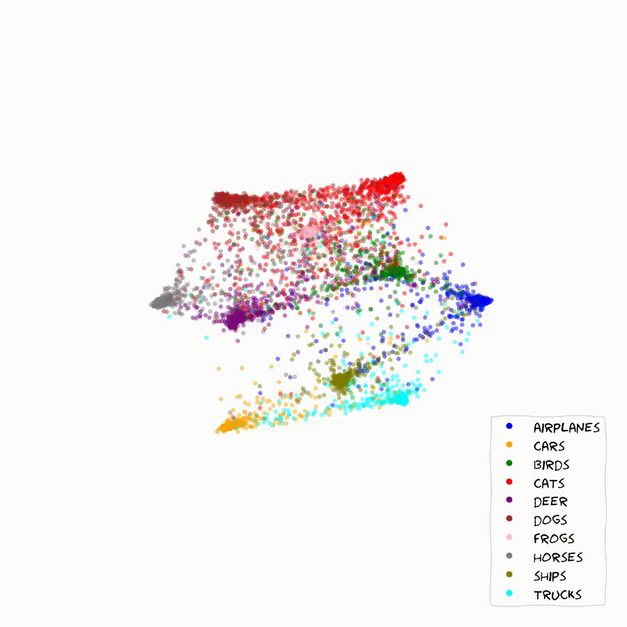
Once we start scaling the feature-dimension we can start getting an intuition for the inner workings of the method. The model learns to arange classes and embedding in order to optimize the relative probabilities of all classes among each other. This often causes chains of embeddings that lie along a smooth probability gradient between classes as seen below.
In these 2D plots, apart from the location of the embeddings of the validation set, I can show the contours of the learned class distributions, as well as the classification boundaries for arbitrary embeddings in the feature-space.
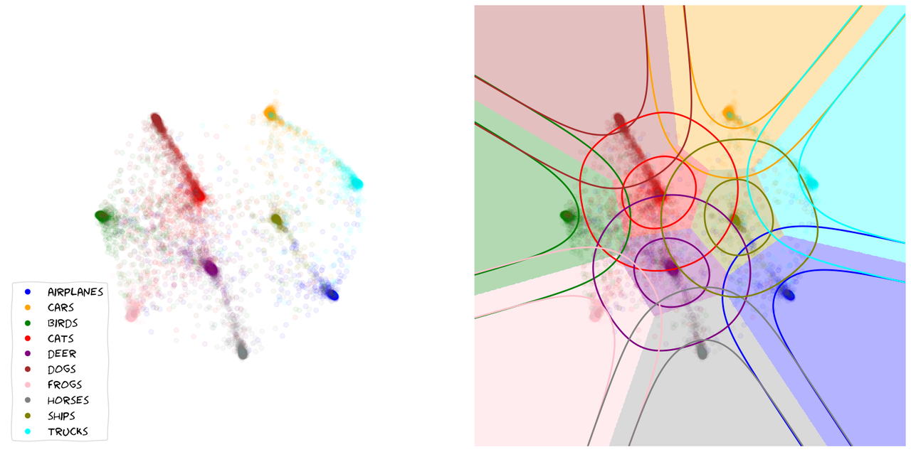
If two classes are easily confounded, we will find their sample embeddings lined up along a gradient of rising certainty towards one of them. Very distinct samples and classes will generally move towards the outer rim of the embedding space, where probabilities get easier to maximize. In the bulk of the embedding space we will generally find classes and embeddings that share features with many other ones.
The Method
So how do we get our embeddings to self-organize so neatly? Simple. We just assume that each class is represented by a multivariate gaussian with the same dimensionality as our feature space. While we could learn mean and standard-deviation for each dimension I found that keeping the scale fixed at 1.0 is usually more stable. So learning the class mean with a single embedding layer is enough. Since we assume that each class is a gaussian in the feature space, for each point in the space we can compute the log-probability for each class which is how we are able to compute that class logits that we need for the cross-entropy loss. To top it all off we also compute the loss between all classes and all class means as a regularization loss. That's it. Pseudocode blow:
img_embs = image_encoder(images)

class_mus = class_encoder(range(n_classes))
class_scale_diag = ones_like(class_mus)

img_logits = log_prob(class_mus, class_scale_diag, img_embs)
class_logits = log_prob(class_mus, class_scale_diag, class_mus)

loss = (
    sparse_categorical_crossentropy(y_true, img_logits)
    + sparse_categorical_crossentropy(range(n_classes), class_logits)
) / 2
Show me the Numbers!
Ok, ok! I see you're not interested in fancy explanantions and just want a number on a standard benchmark dataset with our method in bold. There it is!
The numbers you're looking at have been produced by running an unoptimized training of a ResNet18.
If you want me to run evaluations of bigger models on more serious datasets, help a GPU-poor fella out and hire me in your research lab!😉
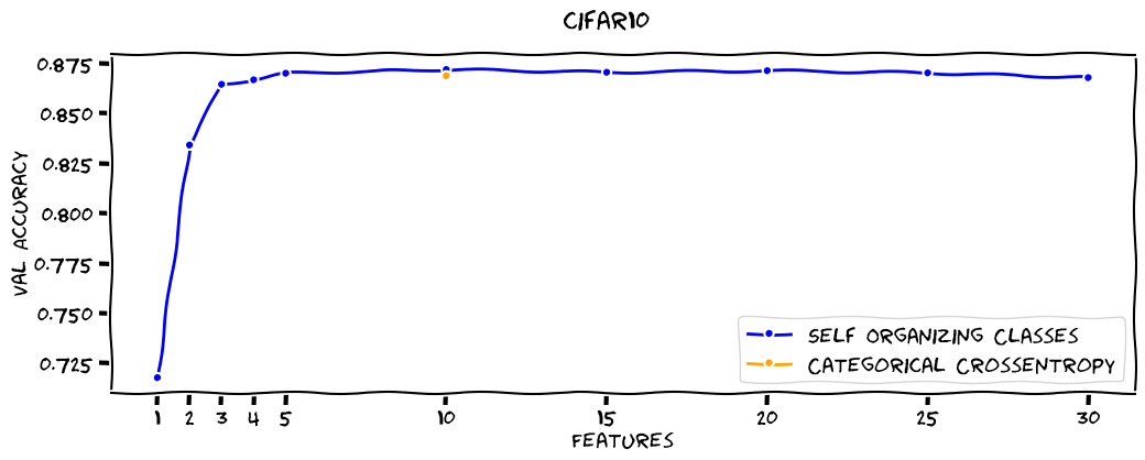
CIFAR10
On average SOC-Embeddings are about as good as Categorical Crossentropy with one feature per class, but in this cherry picked results we beat it of course:
| Loss Type | Features | Val Accuracy |
|---|---|---|
| Categorical Crossentropy | 10 | 86.90% |
| Self Organizing Classes | 1 | 71.80% |
| Self Organizing Classes | 2 | 83.44% |
| Self Organizing Classes | 3 | 86.47% |
| Self Organizing Classes | 4 | 86.70% |
| Self Organizing Classes | 5 | 87.03% |
| Self Organizing Classes | 10 | 87.21% |
| Self Organizing Classes | 15 | 87.07% |
| Self Organizing Classes | 20 | 87.15% |
| Self Organizing Classes | 25 | 87.05% |
| Self Organizing Classes | 30 | 86.81% |
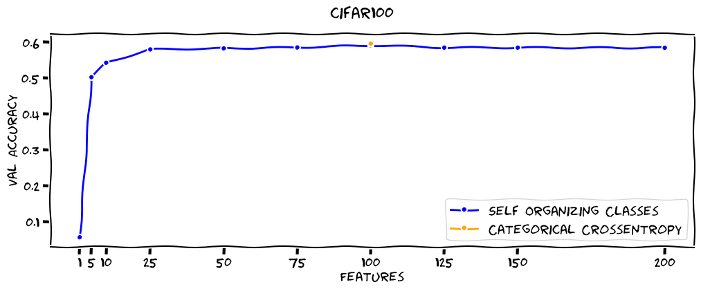
CIFAR100
On Cifar100 SOC-embeddings perform a bit worse so let's give the win to the Categorical Crossentropy with one feature per class here!
| Loss Type | Features | Val Accuracy |
|---|---|---|
| Categorical Crossentropy | 100 | 59.65% |
| Self Organizing Classes | 1 | 5.71% |
| Self Organizing Classes | 5 | 50.32% |
| Self Organizing Classes | 10 | 54.33% |
| Self Organizing Classes | 25 | 58.06% |
| Self Organizing Classes | 50 | 58.34% |
| Self Organizing Classes | 75 | 58.59% |
| Self Organizing Classes | 100 | 59.21% |
| Self Organizing Classes | 125 | 58.55% |
| Self Organizing Classes | 150 | 58.54% |
| Self Organizing Classes | 200 | 58.49% |
Why are SOC-Embeddings exciting?
- Firstly SOC-embeddings are a unification of classification and embeeding models. Previously you had to decide wether you wanted to do classification or embedding. Now you can use the same model for both without modification.
Want to introduce a new class? You can keep the image-model frozen and just train the cheap class-embedding model to find the class location. - SOC-embeddings are neat because they don't force the model to output log-probabilities but coordinates in euclidian space. This does not push the model towards outputting infinities and could lead to more stable gradients.
- You can tune your output dimensionality to your needs. As shown above you can get very close to the original performance while only using a fraction of the original features. This can decrease the dimensionality of your outputs and the cost of computing them significantly while retaining most of the original performance.
Endless possibilities:
- SOC-Clip: Go for it! Just train to learn pairwise means. Clusters of similar objects will emerge.
- SOC-LLM: Easy! Long gone are the times of 52K output dimensions. Just output your embeddings.
- SOC-Attention: Attention has an \(O(n^2 \cdot d + n \cdot d^2)\) complexity right? So let's just reduce the \(d\) ! Squared gains!🚀
- Dense SOC-Layers: Who says we can't use the logits as features again. Go do it!
What other ideas do you have? Let me know on Xitter or LinkedIn! #soc-embeddings
How can YOU train SOC-Embeddings?
Using the gist below you can train SOC-Embedding models like any other Keras model.
from soc_embedding_model import get_soc_model

# prepare dataset and optimizer here...

soc_model = get_soc_model(INPUT_SHAPE, N_CLASSES, EMBEDDING_DIMS)

soc_model.compile(optimizer=optimizer)

soc_model.fit(train_ds, validation_data=val_ds, epochs=EPOCHS)
Expand code to get started
or check out the repo here.
Acknowledgements
- This research was in part supported by Google's TPU Research Cloud.
- Thanks to TensorFlow Probability the implementation of this idea was much easier.
- Credit for the xkcd-font goes to the fantastic Randall Munroe.
- In order to facilitate the visualization of gradients and densities, this blogpost is best consumed to the music it was written to.
Did you find this article helpful for your own research? Please cite it as follows:
@misc{pisoni2023soc_embeddings,
      title={Decoupling Features and Classes with Self-Organizing Class Embeddings},
      url={https://www.rpisoni.dev/posts/self-organizing-class-embeddings/},
      author={Raphael Pisoni},
      year={2023},
}